SOLVING PARTIAL DIFFERENTIAL EQUATIONS BY FACTORING
vertex and slope of linear equation,
adding subtracting dividing multiplying scientific notation worksheet,
vertex and slope of linear graph ,
TI89 quadratic equation solver method
Thank you for visiting our site! You landed on this page because you entered a search term similar to this: solving partial differential equations by factoring.
We have an extensive database of resources on solving partial differential equations by factoring. Below is one of them. If you need further help, please take a look at our software "Algebrator", a software program that can solve any algebra problem you enter!
One will see that the very existence of the eigenvalue spectrum of
 on the unit sphere hinges on this fact.
For this reason, the extension of this algebraic method is considerably more
powerful. It yields not only the basis for each eigenspace of
, but also the actual value for each allowed degenerate
eigenvalue. on the unit sphere hinges on this fact.
For this reason, the extension of this algebraic method is considerably more
powerful. It yields not only the basis for each eigenspace of
, but also the actual value for each allowed degenerate
eigenvalue.
Global Analysis: Algebra
Global analysis deals with the solutions of a differential equation
``wholesale''. It characterizes them in relationship to one another
without specifying their individual behaviour on their domain of
definition. Thus one focusses via algebra, linear or otherwise, on
``the space of solutions'', its subspaces, bases etc.
Local analysis (next subsubsection), by contrast, deals with the solutions
of a differential equation ``retail''. Using differential calculus,
numerical analysis, one zooms in on individual functions and characterizes
them by their local values, slopes, location of zeroes, etc.
1. Factorization
The algebraic method depends on factoring
into a pair of first order operators which are adjoints of each other.
The method is analogous to factoring a quadratic polynomial, except
that here one has differential operators
 and
and
 instead of the variables instead of the variables  and and  .
Taking our cue from Properties 16 and 17, one attempts
However, one immediately finds that this factorization yields .
Taking our cue from Properties 16 and 17, one attempts
However, one immediately finds that this factorization yields
 for a cross
term. This is incorrect. What one needs instead is for a cross
term. This is incorrect. What one needs instead is
 . This
leads us to consider . This
leads us to consider
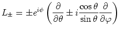
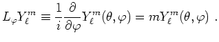
Here we have introduced the self-adjoint operator
It generates rotations around the polar axis of a sphere. This operator,
together with the two mutually adjoint operators
are of fundamental importance to the factorization method of solving
the given differential equation. In terms of them the factorized
Eq.(5.135) and its complex conjugate have the form
 |
(5136) |
This differs from Eq.(5.16),
(Property 17 on page ), the
factored Laplacian on the Euclidean plane.
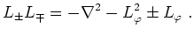
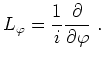
2. Fundamental Relations
In spite of this
difference, the commutation relations corresponding to
Eqs.() are all the same, except one. Thus, instead
of Eq.(5.19), for a sphere one has
![$\displaystyle [L_+,L_-]=2L_\varphi~.$](img3906_1.png) |
(5137) |
This is obtained by subtracting the two
Eqs.(5.136). However, the commutation
relations corresponding to
the other two equations remain the same. Indeed, a little algebraic
computation yields
or
![$\displaystyle [L_\varphi, L_\pm]= \pm L_\pm ~.$](img3908_1.png) |
(5138) |
Furthermore, using Eq.(5.136) one finds
The last equality was obtained with the help of
Eqs.(5.137) and (5.138).
Together with the complex conjugate of this equation, one has therefore
![$\displaystyle [\nabla^2,L_\pm]=0~.$](img3915_1.png) |
(5140) |
In addition, one has quite trivially
![$\displaystyle [\nabla^2,L_\varphi]=0$](img3916_1.png) |
(5141) |
The three algebraic relations,
Eqs.(5.137)-(5.138)
and their consequences,
Eq.(5.140)-(5.141), are the
fundamental equations from which one deduces the allowed degenerate
eigenvalues of Eq.(5.132)
as well as the corresponding normalized eigenfunctions.
3. The Eigenfunctions
One starts by considering a function
 which is a simultaneous
solution to the two eigenvalue equations which is a simultaneous
solution to the two eigenvalue equations
This is a consistent system, and it is best to postpone until later
the easy task of actually exhibiting non-zero solutions to it. First
we deduce three properties of any given solution
.
The first property is obtained by applying the operator  to this solution. One finds that
Similarly one finds
Thus
 and and
 are again eigenfunctions of are again eigenfunctions of
 , but having eigenvalues , but having eigenvalues  and and  . One is, therefore,
justified in calling and . One is, therefore,
justified in calling and  raising and
lowering operators.
The ``raised'' and ``lowered'' functions raising and
lowering operators.
The ``raised'' and ``lowered'' functions
 have the additional property that they are still
eigenfunctions of belonging to the same eigenvalue have the additional property that they are still
eigenfunctions of belonging to the same eigenvalue  .
Indeed, with the help of Eq.(5.140) one finds
Thus, if
belongs to the eigenspace of ,
then so do
and
. .
Indeed, with the help of Eq.(5.140) one finds
Thus, if
belongs to the eigenspace of ,
then so do
and
.
4. Normalization and the Eigenvalues
The second and third properties concern the normalization of
 and the allowed values of .
One obtains them by examining the sequence of squared norms
of the sequence of eigenfunctions and the allowed values of .
One obtains them by examining the sequence of squared norms
of the sequence of eigenfunctions
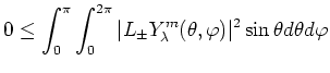
All of them are square-integrable. Hence their norms are non-negative.
In particular, for  one has one has
This is the second property. It is a powerful result for two reasons:
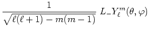
First of all, if
 has been normalized to unity, then so
will be has been normalized to unity, then so
will be
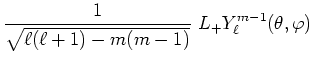
![$\displaystyle \frac{1}{[\lambda - m(m\pm 1)]^{1/2}} L_\pm Y_\lambda^m(\theta,\varphi) \equiv Y_\lambda^{m\pm 1}(\theta,\varphi)$](img3941_1.png) |
(5143) |
This means that once the normalization integral has been worked out
for any one of the
's, the already normalized
 are given by
Eq.(5.143); no additional
normalization integrals need to be evaluated. By repeatedly applying
the operator are given by
Eq.(5.143); no additional
normalization integrals need to be evaluated. By repeatedly applying
the operator  one can extend this result to one can extend this result to
 , ,
 , etc. They all are already normalized if
is. No extra work is necessary. , etc. They all are already normalized if
is. No extra work is necessary.
Secondly, repeated use of the relation (5.142)
yields
This relation implies that for sufficiently large integer  the
leading factor in square brackets must vanish. If it did not, the
squared norm of the
leading factor in square brackets must vanish. If it did not, the
squared norm of
 would become negative. To
prevent this from happening, must have very special values.
This is the third property: The only allowed values of are
necessarily
(Note that would become negative. To
prevent this from happening, must have very special values.
This is the third property: The only allowed values of are
necessarily
(Note that
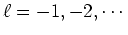 would give nothing new.) Any other
value for would yield a contradiction, namely a negative
norm for some integer . As a consequence, one has the result
that for each allowed eigenvalue there is a
sequence of eigenfunctions would give nothing new.) Any other
value for would yield a contradiction, namely a negative
norm for some integer . As a consequence, one has the result
that for each allowed eigenvalue there is a
sequence of eigenfunctions
 |
(5144) |
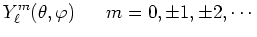
(Nota bene: Note that these eigenfunctions are now labelled by
the non-negative integer  instead of the corresponding
eigenvalue .) Of particular interest are the two
eigenfunctions instead of the corresponding
eigenvalue .) Of particular interest are the two
eigenfunctions
 and and
 . The squared norm of . The squared norm of
 ,
is not positive. It vanishes. This implies that ,
is not positive. It vanishes. This implies that
 |
(5145) |
In other words,
 and all subsequent members of the
above sequence, Eq.(5.144) vanish, i.e.
they do not exist. Similarly one finds that and all subsequent members of the
above sequence, Eq.(5.144) vanish, i.e.
they do not exist. Similarly one finds that
 |
(5146) |
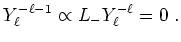
Thus members of the sequence below
do not exist either.
It follows that the sequence of eigenfunctions corresponding to
 is finite. The sequence has only is finite. The sequence has only  members, namely
for each integer . The union of these sequences forms a semi-infinite
lattice in the members, namely
for each integer . The union of these sequences forms a semi-infinite
lattice in the  as shown in
Figure 5.21. as shown in
Figure 5.21.
Figure 5.21:
Lattice of eigenfunctions (spherical hamonics) labelled
by the angular integers and  . Application of the raising operator
increases by . Application of the raising operator
increases by  , until one comes to the top of each
vertical sequence (fixed ). The lowering operator
decreases by , until one reaches the bottom.
In between there are exactly lattice points, which express
the ()-fold degeneracy of the eigenvalue
.
There do not exist any harmonics above or below
the dashed boundaries. , until one comes to the top of each
vertical sequence (fixed ). The lowering operator
decreases by , until one reaches the bottom.
In between there are exactly lattice points, which express
the ()-fold degeneracy of the eigenvalue
.
There do not exist any harmonics above or below
the dashed boundaries.
|
For obvious reasons it is appropriate to
refer to this sequence as a ladder with elements, and
to call
the top, and
the
bottom of the ladder. The raising and lowering operators
are the ladder operators which take us up and down the
 -element ladder. It is easy to determine the elements -element ladder. It is easy to determine the elements
 at the top and the bottom, and to use the ladder
operators to generate any element in between. at the top and the bottom, and to use the ladder
operators to generate any element in between.
5. Orthonormality and Completeness
The operators
 form a complete set of commuting
operators.
This means that their eigenvalues
serve as sufficient labels to uniquely identify each of
their (common) eigenbasis elements for the vector space of solutions
to the Hermholtz equation form a complete set of commuting
operators.
This means that their eigenvalues
serve as sufficient labels to uniquely identify each of
their (common) eigenbasis elements for the vector space of solutions
to the Hermholtz equation
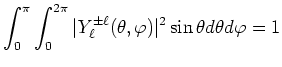
on the two-sphere. No additional labels are necessary. The fact that
these operators are self-adjoint relative to the inner product,
Eq.(5.134), implies that these
eigenvectors (a.k.a spherical harmonics) are orthonormal:
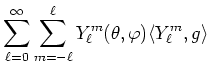
The semi-infinite set
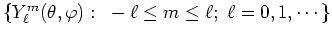 is a basis for the vector space of functions
square-integrable on the unit two-sphere. Let is a basis for the vector space of functions
square-integrable on the unit two-sphere. Let
 be
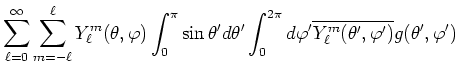
any such function. Then be
any such function. Then
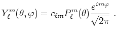
In other words, the spherical harmonics are the basis elements for a
generalized double Fourier series representation of the function
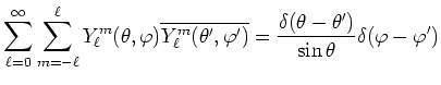
. If one leaves this function unspecified,
then this completeness relation can be restated in the equivalent
form
in terms of the Dirac delta functions on the compact domains
 and and
 . .
Local Analysis: Calculus
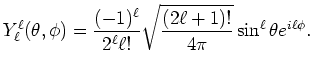
What is the formula for a harmonics
 ?
An explicit functional form determines the graph, the location of its
zeroes, and other aspects of its local behaviour. ?
An explicit functional form determines the graph, the location of its
zeroes, and other aspects of its local behaviour.
1. Spherical Harmonics: Top and Bottom of the Ladder
Each member of the ladder sequence satisfies the differential equation
Consequently, all eigenfunctions have the form
 |
(5147) |
Here
 is a normalization factor.
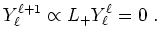
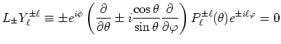
The two eigenfunctions
and
at the top and the bottom of the ladder satisfy Eqs.(5.145)
and (5.146) respectively, namely is a normalization factor.
The two eigenfunctions
and
at the top and the bottom of the ladder satisfy Eqs.(5.145)
and (5.146) respectively, namely
 |
(5148) |
It is easy to see that their solutions are
The normalization condition
implies that
 |
(5149) |
The phase factor  is not determined by the normalization.
Its form is chosen so as to simplify the to-be-derived formula for the
Legendre polynomials, Eq.(5.153). is not determined by the normalization.
Its form is chosen so as to simplify the to-be-derived formula for the
Legendre polynomials, Eq.(5.153).
2. Spherical harmonics: Legendre and Associated Legendre
polynomials
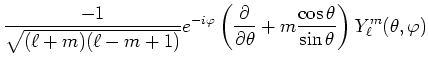
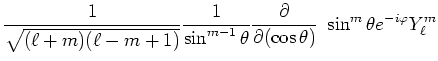
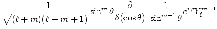
The functions
 are obtained by applying the
lowering operator to are obtained by applying the
lowering operator to
 . A systematic
way of doing this is first to apply repeatedly the lowering relation . A systematic
way of doing this is first to apply repeatedly the lowering relation
to
until one obtains the azimuthally
invariant harmonic
 . Then
continue applying this lowering relation, or alternatively the raising
relation . Then
continue applying this lowering relation, or alternatively the raising
relation
until one obtains the desired harmionic
.
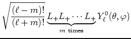
The execution of this two-step algorithm reads as follows:
Step 1: Letting
 , apply Eq.(5.150)
times and obtain , apply Eq.(5.150)
times and obtain
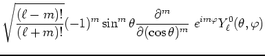
which, because of Eq.(5.147), is independent of
 . Now let . Now let  , use Eq.(5.149),
and obtain , use Eq.(5.149),
and obtain
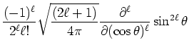
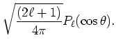
The polynomials in the variable

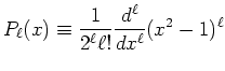 |
(5153) |
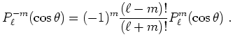
are called the Legendre polynomials. They have the property
that at the North pole they have the common value unity, while at the
South pole their value is  whenever whenever  is an even
polynomial and is an even
polynomial and  whenever it is odd:
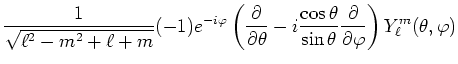
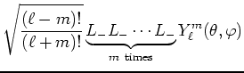
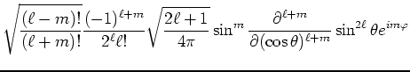
Step 2: To obtain the harmonics having positive azimuthal integer
, apply the raising operator times to whenever it is odd:
Step 2: To obtain the harmonics having positive azimuthal integer
, apply the raising operator times to  . With the
help of Eq.(5.151) one obtains (for
) . With the
help of Eq.(5.151) one obtains (for
)
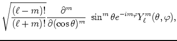
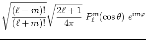
The polynomials in the variable
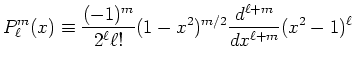 |
(5155) |
are called the associated Legendre polynomials.
Inserting Eq.(5.154) into
Eq.(5.132), one finds that they satisfy the differential equation
Also note that
 satisfies the same differential
equation. In other words, satisfies the same differential
equation. In other words,
 and and
 must be
proportional to each other. (Why?) Indeed, must be
proportional to each other. (Why?) Indeed,
 |
(5156) |
|


![$\displaystyle \left[ \frac{1}{\sin\theta} \frac{d}{d\theta} \sin\theta
\frac{d...
...heta}+\ell(\ell+1)-\frac{m^2}{\sin^2\theta} \right]
P^{m}_\ell(\cos\theta)=0~.
$](img4017_1.png)